APh 162 Biological Physics LaboratoryDavid Van Valen Michael Amori |
|||||||||||||||||||||||||||||||||||||||||||||||||||||||||||||||||||||||||||||||||||||||||
Sizes Rates DNA Science |
The Size of Things
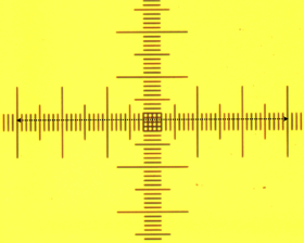
The goal of this segment of the course was to get a feel for the size of biological organisms. The first step was to calibrate our microscopes to obtain a conversion from voxels to an actual length. To do this, we viewed essentially looked at a ruler with different objectives and measured known lengths in terms of voxels.
Figure 1: Calibrating the microscope This calibration gave us the conversion
With these conversion factors, we then examined three organisms: Stentor, E. Coli, and C. Elegans. Stentor
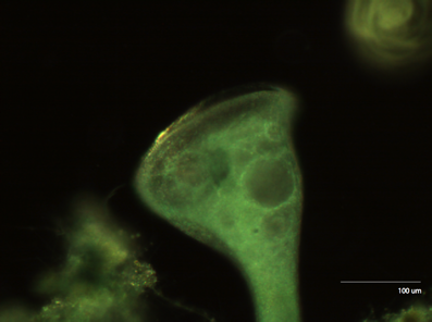
The first organism we looked at was Stentor, one of the largest unicellular organisms available.
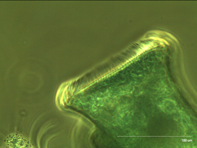
Figure 2: Stentor at 10x Upon closer inspection, we can see the collections of cilia (cirri) that stentor uses to generate the vortices that propel food into its mouth.
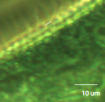
Figure 3: Stentor at 20x Zooming in, we can estimate the spacing between cirri to be about 12.2 voxels, or 3.146 um.
Figure 4: Estimating the distance between
cirri E. Coli
The second species we examined was E. Coli, which has been the benchmark organism for this course. E. Coli has a remarkable ability to utilize plasmids to alter its pathogenicity. The bacteria we observed were, of course, devoid of any such modifications.
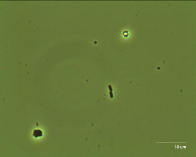
Figure 5: E. Coli on a glass slide.
Photograph taken at 100x E. Coli is too small to be properly visualized at less than 100x. In order to use the 100x objective, we had to place a drop of oil between the objective and our sample. The oil has the same refractive index as the glass coverslip and the objective, and serves to remove coverslip-air and air-objective interfaces to allow for higher resolution. The images we captured appear to have been taken just after a cell division. The most interesting measurement we can make is the size of E. Coli. One cell is approximately 47.67 voxels, or 2.46 um. C. Elegans
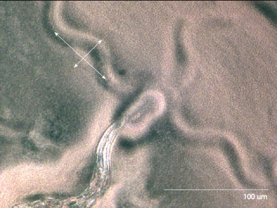
The third species we observed was C. Elegans. http://snowdome.caltech.edu/aph162/David and Michael/worm2.avi By looking at the indentation the worm makes in the media, we can measure its amplitude and its wavelength. |
||||||||||||||||||||||||||||||||||||||||||||||||||||||||||||||||||||||||||||||||||||||||
|
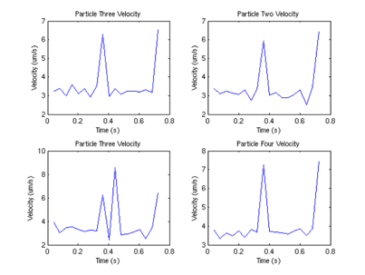
Sperm |
Velocity (um/s) |
|
1 |
3.5862 |
|
2 |
3.4445 |
|
3 |
3.8090 |
|
4 |
4.0589 |
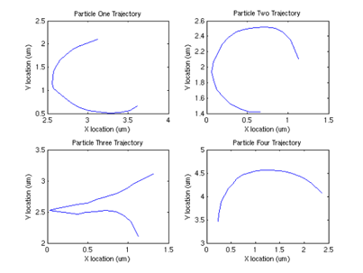
Interestingly, we can also compute the correlation between velocities of different sperm.
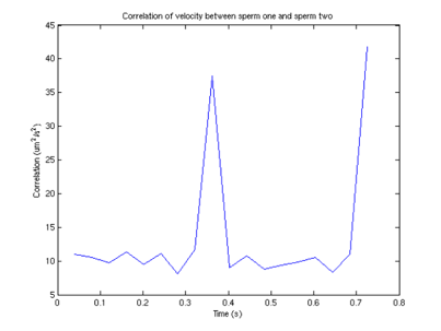
Figure 9: Velocity correlation between
sperm 1 and sperm 2
From this graph, we can see that surprisingly (although not surprising if one looks at the data) that the velocities are correlated, and there appears to be a periodicity of about .4 seconds in the velocity. One possible explanation (courtesy of Tristan Ursell) is that the sperm are not free in solution. It is possible that the flagella of the sperm are tethered to the bottom of the glass slide. This would account for the circular motion we see, which would also explain the correlation in velocities.
To calculate the rate of ATP consumption, we will assume that the viscous forces that act on the sperm can be modeled by Stoke’s law,
where ![]() is the viscosity, r is the radius of
the sperm, and v is it’s velocity. To keep a constant velocity, ATP must be
converted to ADP to produce enough energy to oppose the work being done by
the viscous fource. So the energy per second needed is
is the viscosity, r is the radius of
the sperm, and v is it’s velocity. To keep a constant velocity, ATP must be
converted to ADP to produce enough energy to oppose the work being done by
the viscous fource. So the energy per second needed is
Using the values,
|
Quantity |
Value |
|
|
8.90*10-4 Ns/m2 |
|
R |
5.79 um |
we see that the energy expended per second is
|
Sperm |
Energy/second (J/s) |
|
1 |
1.249*10-18 |
|
2 |
1.153*10-18 |
|
3 |
1.409*10-18 |
|
4 |
1.600*10-18 |
The energy generated from the hydrolysis of ATP is 7.3 kcal/mol, which is 5.07*10-20 J/molecule. Using this value, the ATP consumed by the sperm per second is
|
Sperm |
ATP/second (molecules/s) |
|
1 |
24.6 |
|
2 |
22.7 |
|
3 |
27.8 |
|
4 |
31.6 |
So an average of 26.7 ATP/second is consumed to propel the sperm through the aqueous media.
DNA Science
The third segment of the course focused on DNA science and the protocols behind manipulating genomes. The goal for this part was simple: we wanted to create bacterial cell that expressed lacZ with a tetracycline inducible promoter. The pieces we started with were
- A vector with an gene for kanamycin resistance and GFP
- DNA from E Coli and plasmids that contained lac Z
The protocol was essentially cut and paste. We first used restriction enzymes to cut our vector, then ran the products through a agarose gel using electrophoresis to purify the portion that had the antibiotic resistance.
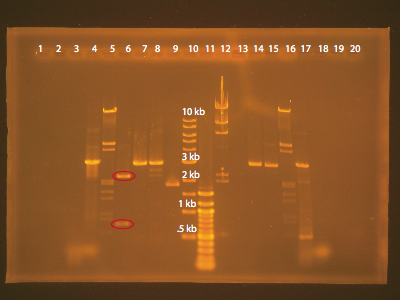
The contents of the lanes are as follows
|
Lane |
Content |
|
1 |
None |
|
2 |
None |
|
3 |
PCR from E-Coli |
|
4 |
PCR from purified plasmid |
|
5 |
Lambda-DNA + HindIII + EcoR1 |
|
6 |
PZE21-GFP + KpnI + HindIII |
|
7 |
PZE21-GFP + KpnI |
|
8 |
PZE21-GFP + HindIII |
|
9 |
Uncut PZE21-GFP plasmid |
|
10 |
1 kb ladder |
|
11 |
100 bp ladder |
|
12 |
Lambda-DNA + HindIII |
|
13 |
PZE21-GFP + KpnI + HindIII |
|
14 |
PZE21-GFP + KpnI |
|
15 |
PZE21-GFP + HindIII |
|
16 |
Lambda-DNA + HindIII + EcoR1 |
|
17 |
PCR from purified plasmid |
|
18 |
PCR from E-Coli |
|
19 |
None |
|
20 |
None |
The key lanes that we had to analyze were lanes 6, 7, 8, 9,13, 14, and 15. The goal of this gel was to isolate the band that contains our original vector with the GFP piece cut out. This corresponds to lanes 6 and 13. Lane 6 has two bands, which is what we expect – one corresponds to the vector fragment and the other corresponds to the GFP fragment. Interestingly, lane 13 which should have identical contents is empty, possibly due to an error in loading the gel. A closer look at lane 6 shows that we have one band between 2 kb - 3 kb and another between .5 kb – 1 kb. Analysis with VectorNTI reveals that the vector fragment will be 2900 bp and the GFP fragment will be 700 bp. Hence, the upper band is the vector that we want to isolate.
As a sanity check we can also analyze the other lanes. Lanes 7/14 and 8/15 contain the plasmid cut with a single restriction enzyme. This should yield a linear fragment of about 3600 bp. The ladder places this band around 3 kb, so this makes sense. Lane 9 contains the uncut plasmid. As expected, the circular conformation alters how the DNA polymer travels through the gel, and its band is shifted compared to the linear strands of DNA in lanes 7 and 8. The results of our gel do indeed make sense.
After cutting out the appropriate band to get the GFP-free vector, we then PCR amplified the lacZ region of our DNA using primers that would give us the appropriate sticky ends we needed for ligation. Next, we combined the vector with our lacZ insert with DNA ligase to obtain our desired plasmid. Bacterial cells were then transformed with our plasmid using electroporation, and plated on agarose that contained IPTG and kanamycin. Cells that were successfully transfected with the plasmid should express beta-galactosidase, an enzyme that cleaves IPTG, causing colonies that contain the plasmid to appear blue on the plate.
References
- Wikipedia
- Alberts, Molecular Biology of the Cell
- http://www.neb.com/nebecomm/productsN3232asp