.: Introduction
 |
Microtubules (MT) play a significant role in
almost all stages of mitosis. Their functions include movement of
organelles, transport of vesicles, protein attachment, as well as
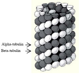
cytoskeleton support. MT is composed of an
a,β-tubulin heterodimer which are similar and approximately 55 kDa MW
each. When the tubulin are polymerized, they are joined from end to
end to form a profilament. 13 profilaments assemble to form a helical
arrangement that forms the MT as shown on the right. It is important
to note that tubulin can be polymerized at both ends in vitro at
different rates where the faster rate is the plus-end and the slower rate is
the minus-end. These dynamic rates have been of particular interest to
biophysicists as they appear to be fundamental to explain cellular
organization. |
| Image courtesy of Cytoskeleton, Inc. |
|
.: Aims
The purpose of our study was to determine the dynamic
instability of microtubule growth using fluorescent microtubules and fluorescent
microscopy. Using methods developed by
Mitchison and
Kirschner, growth will be arrested at multiple time points and MT lengths
will be measured to determine the dynamics of MT polymerization.
Furthermore, the kinetics of MT polymerization will be determined by quantifying
the relationship between MT length and tubulin concentration.
[top]
.: Methods
Tubulin Preparation:
- Using Fluorecent Microtubules Biochem Kit (Cat
#BK007R), concentrations and measurements were pre-determined due to the
fragility of the tubulin protein which begins to degrade when left at room
temperature. Therefore, all mixtures were stored on ice when not in use.
GPEM: General tubulin buffer (GTB) and GTP at 1:100 ration
Non-labeled tubulin: 50 ul @ 250 ug + 40ul of GPEM + 10 ul cushion buffer =
5 mg/mL
Labeled tubulin: 5 ul @ 20 ug + 4 ul of GPEM + 1 ul of cushion buffer = 4mg/mL
To obtain at 30% ratio of non-labeled to labeled tubulin:
3.3 ul of unlabeled tubulin = 16.5 ug
1.7 ul of labeled tubulin = 6.8 ug
--> 4.66 ug/ul
5 ul
29.3 ug
- Put 500 ul of purified H2O into eppendorf and
place on ice.
- Put 100 ul of cold H2O into GTP stock to
reconstitute it and aliquot into 10 ul individual eppendorfs and store at -70
degC.
- Take 99ul of GTB and using 1 ul of one of the GTP aliquots
to make 100 uL of GPEM
- Add 4ul of GPEM and 1ul of cushion buffer to 5 ul of
labeled tubulin.
- Add 40ul of GPEM and 10ul of cushion buffer to 50 ul of
unlabeled tubulin.
- Place 15 eppendorfs into ice and label as "30% labeled
tubulin"
- From (6), take 3.3 ul of diluted unlabeled tubulin and add
to one eppendorf from (7)
- From (5), take 1.7 ul of diluted labeled tubulin and add to
eppendorf from (8)
- Repeat for all 15 aliquots and place on ice.
- In order to store for future use, snap freeze 30% tubulin
mixture by dipping into LN2 with tweezers for approximately 7
seconds and store in -70 degC freezer.
- Dilute taxol into 100 ul of DMSO and aliquot into 12 50uL
2.2mM taxol and store in freezer.
- Prepare antifade by adding 1ml of 50% glycerol and purified
H2O to reconstitute antifade if necessary, then add 50uL of 10x
antifade (AF) to 450ul of GTB and aliquot, store at -70 degC.
[top]
EMCL Concentration Determination
- Put 500 uL of GTB into an eppendorf and heated it in
waterbath at 35 degC for 15 minutes.
- Added 5ul of 2mM Taxol to GTB.
- Placed one aliquot of 30% labeled tubulin (46.6 mM
concentration) into waterbath at 35 degC for 10 minutes.
- At 10 min, withdraw eppendorf from water bath and add 100
ul of GTB+Taxol mixture to arrest polymerization (both due to Taxol and due to
dilution).
- Take 1uL of (4) and add 10 uL of antifade.
- Take 7uL of (5) and place on a slide, place coverslip, and
seal edges with melted wax.
- Add a drop of microscope oil and view at 100x on the Zeiss
Axio microscope using filter 5 (TexRed) and with fluorescence on. Be
careful not to keep fluorescence on for long as it will cause depolymerization
of the microtubules.
- Repeat steps 5-7 except with 1uL, 2uL, 3uL, 5uL of EMCL and
view to determine optimal EMCL concentration. 2uL EMCL seemed to work
best.
[top]
Microtubule Polymerization and Visualization
- The following concentrations of 30% labeled MT were
prepared:
46.6 uM = 0.5 uL of MT, No GTB added (x5)
20.0 uM = 2 uL of MT, 3 uL of GTB (x5)
10.0 uM = 1 uL of MT, 4 uL of GTB (x5)
5.0 uM = 0.5 uL of MT, 4.61 uL of GTB (x5)
2.5 uM = 0.5 uL of MT, 8.82 ul of GTB (x3), aliquot to 5 uL each
1 uM = 0.5 uL of MT, 22.8 uL of GTB (x1),
aliquot to 5 uL each
- Place each concentration in water bath for the following
times: 5, 10, 15, 20, and 30 minutes. In the 46.6uM solution, times were
1, 2, 5, 10, 20, and 30 minutes.
- When time has been reached, add 100 ul of GTB+Taxol mixture
to arrest polymerization.
- Take 1uL of (3) and add 10 uL of antifade and 2uL of EMCL.
- Take 7uL of (4) and place on a slide, place coverslip, and
seal edges with melted wax.
- Add a drop of microscope oil and view at 100x on the Zeiss
Axio microscope using filter 5 (TexRed) and with fluorescence on. Be
careful not to keep fluorescence on for long as it will cause depolymerization
of the microtubules.
- Acquire fluorescent images with AxioCam and using
AxioVision v4.4 to capture images.
- Multiple locations throughout the slide were selected for a
total of five images per concentration per time point.
- 150ms exposure time was used for all images.
- Save images as 16-bit images and store on
snowdome.caltech.edu/AEK.
[top]
Data Analysis
- MT images all time points from 20uM and 46.6uM
concentrations were analyzed.
- Manual measurement of MT thickness was made to ensure that
all MT are the same width.
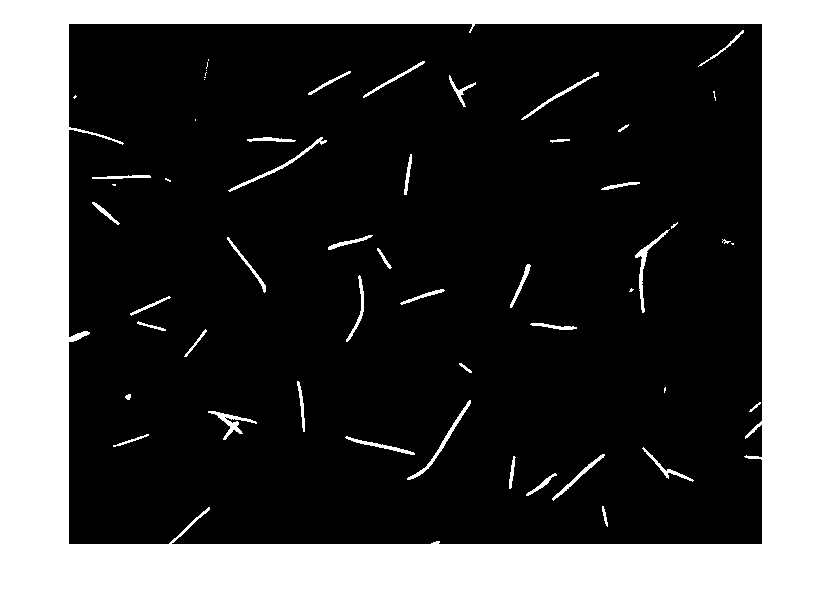
- Generated code in
Matlab to measure MT area for each concentration and at each time point.
Assuming that (2) is true for all MT, then area is proportional to length.
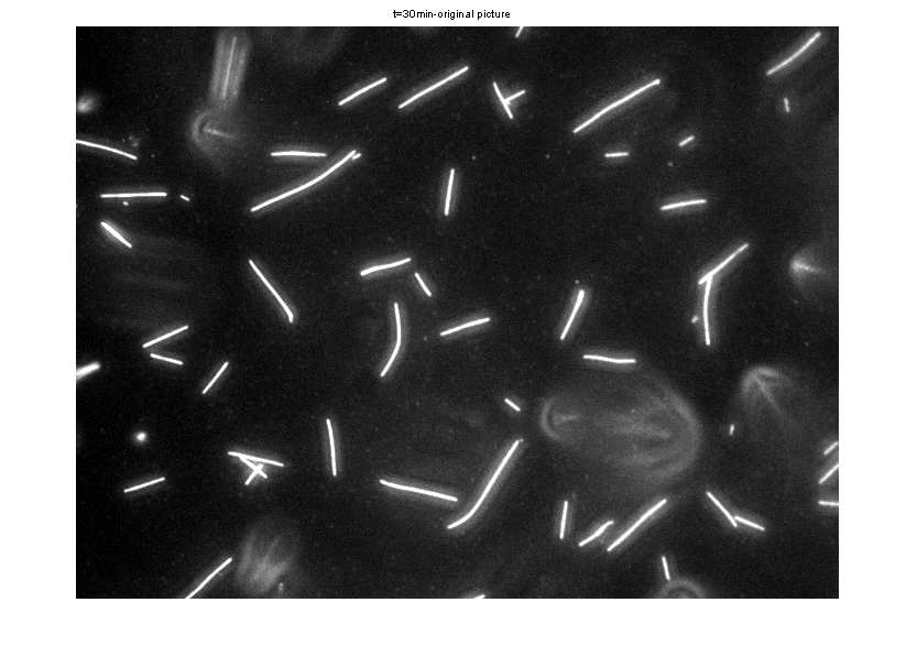
Original Image before Matlab processing
Segmented image after Matlab image processing
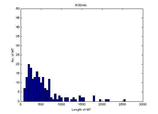
- Bins were set at lengths of 50 and analysis was restricted
to 100<area<3000 pixels to eliminate background noise and out-of-focus
fluorescent MT.
- Lengths were then plotted versus time.
- Concentration was plotted vs. lengths.
[top]
.: Results
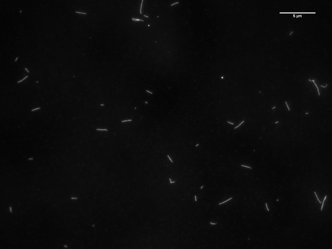
Microtubule Images and Length Measurements at 46.6 uM
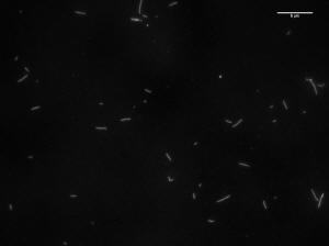

Image of 47uM concentration taken at 1 minute
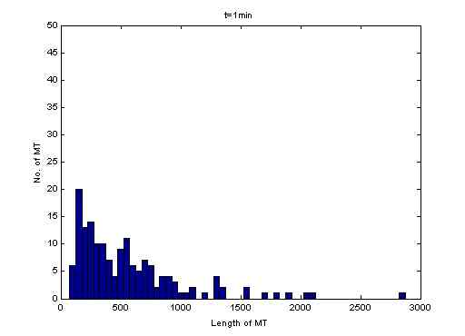
Histogram of MT length at 1 minute
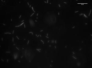
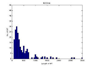
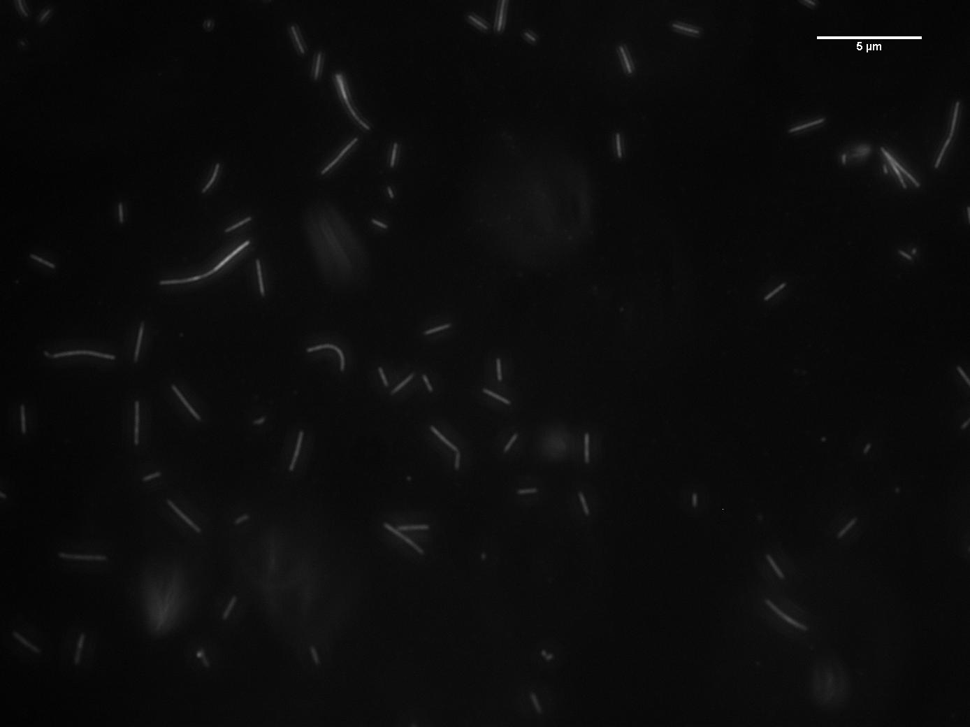
Image of 47uM concentration taken at 2 minutes
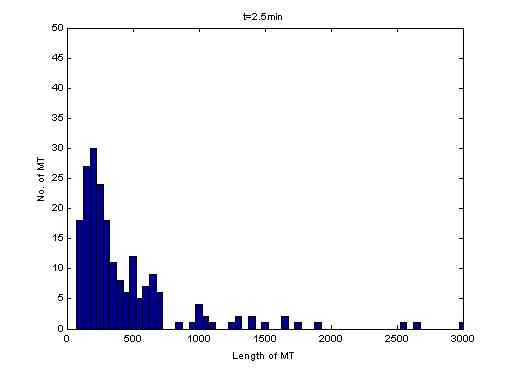
Histogram of MT length at 2 minutes
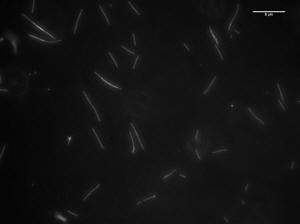
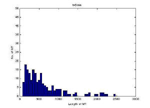
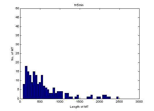
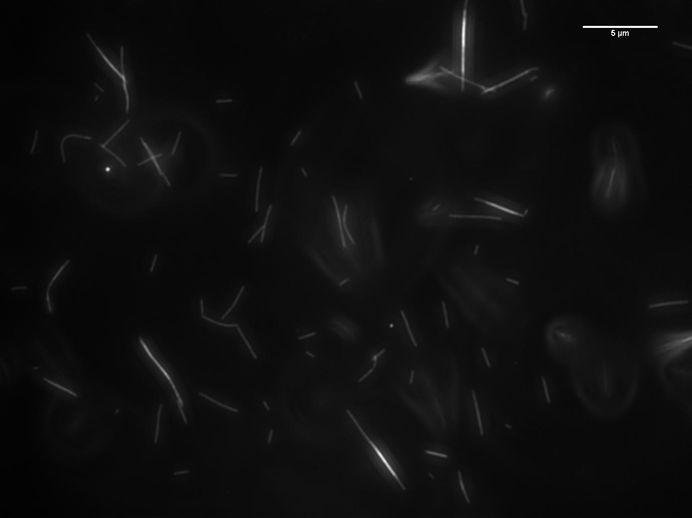
Image of 47uM concentration taken at 5 minutes
Histogram of MT length at 5 minutes

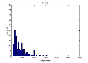
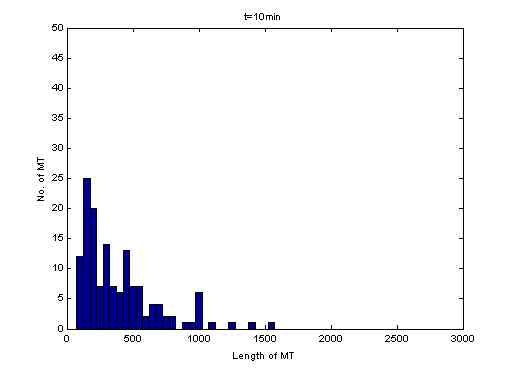
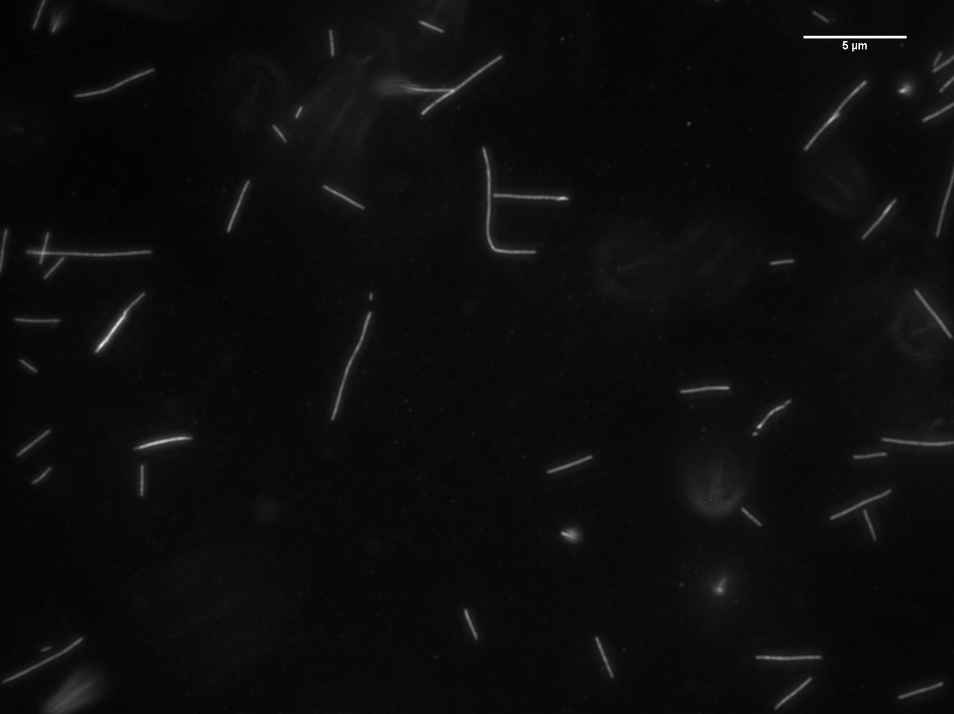
Image of 47uM concentration taken at 10 minutes
Histogram of MT length at10 minutes
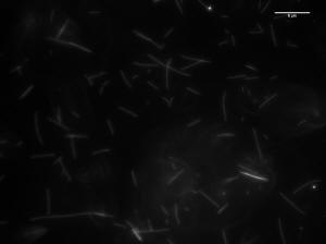
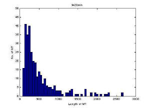
Image of 47uM concentration taken at 20 minutes
Histogram of MT length at 20 minutes
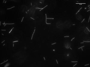

Image of 47uM concentration taken at 30 minutes
Histogram of MT length at 30 minutes
[top]
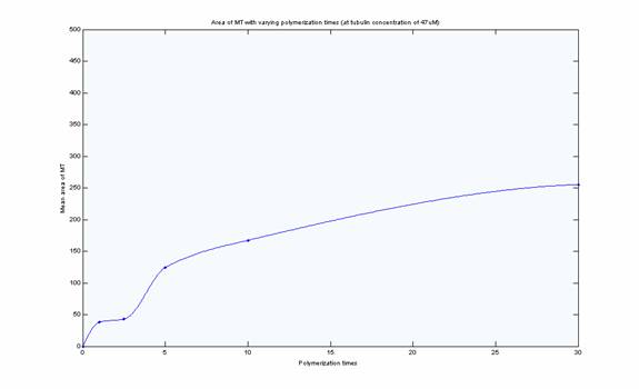
Mean MT length vs. Polymerization Time for 47uM
MT length appeared to reach steady state after 5 minutes at
this concentration based on the histograms and visual inspection of the
images. Mean length however does not reflect steady-state as
demonstrates in the plot versus time. This is likely due to uneven
sampling of the population of microtubules in the images. One source of error
was that at high concentration there were a significant number of MT in the
field of view and therefore significant time was spent focusing the images.
The longer the fluorescence is on, the more MT are degraded.
Furthermore, at high concentration there is a shearing effect which may also
be reflected in the lack of steady-state.
[top]
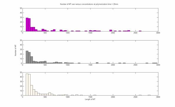
MT Lengths over time at 20uM
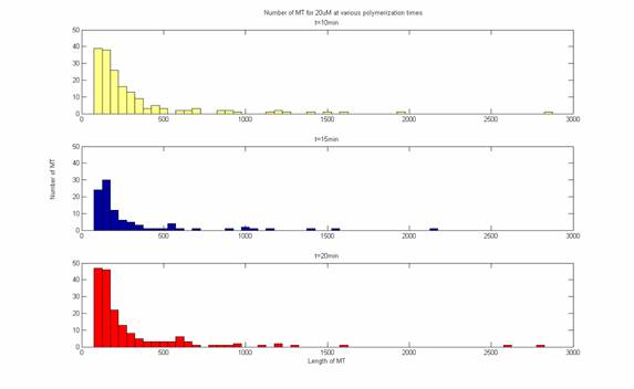
MT Lengths
at 20 uM
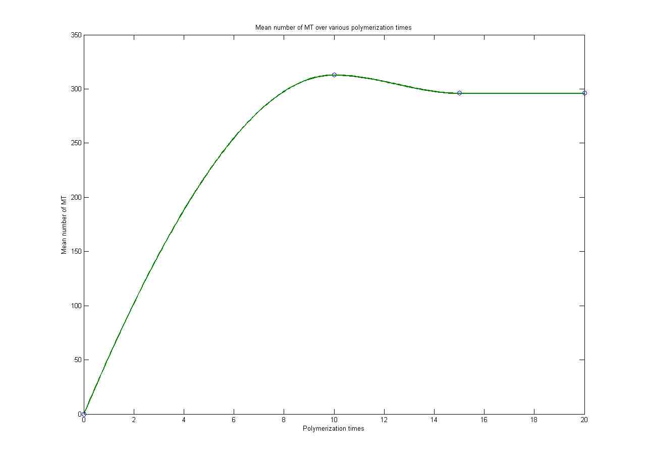
MT length over time at 20uM
At 20uM steady state is achieved after 10 minutes. This
demonstrates the dynamic instability of MT growth.
[top]
Growth Rate at Different Concentrations:
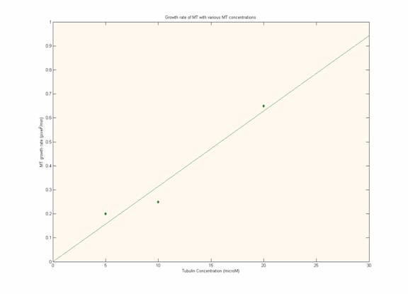
These figures clearly demonstrate that as tubulin
concentration increases, the growth rate increases linearly. The line
fit was a least squares fit. This reflects a simple first-order rate
equation from which the rates of microtuble assembly can be calculated.
Unfortunately, we did not measure depolymerization rates which would need to
be taken into consideration for accurate kinetic calculations.
Images were acquired (but now shown) of concentrations at
10uM and lower because there was little to no microtubules present in the
slide. We believe that this error arises from the low volumes of labeled
tubulin that we were pipetting into the polymerization solution. It is
likely that the tubulin stuck to the sides of the pipette tip and were not
successfully transferred to the ependorf tubes. At higher
concentrations, the small loss of tubulin would not have a siginficant effect
but at low concentrations, the loss can significant, causing the solution to
fall under the critical concentration necessary for polymerization.
.: Conclusion
We have successfully replicated the Mitchison and Kirschner
study of the dynamic instability of microtubule growth. The data reflects
steady-state dynamics and the kinetics that were obtained with electron
microscopy in the earlier work.
[top]
Web site contents © Copyright AEK 2006, All rights reserved.
Website templates
|